


 89 / 743

Dynamic Data Analysis – v5.12.01 - © KAPPA 1988-2017
Chapter
3 – P ressure Transient Analysis (PTA)- p89/743
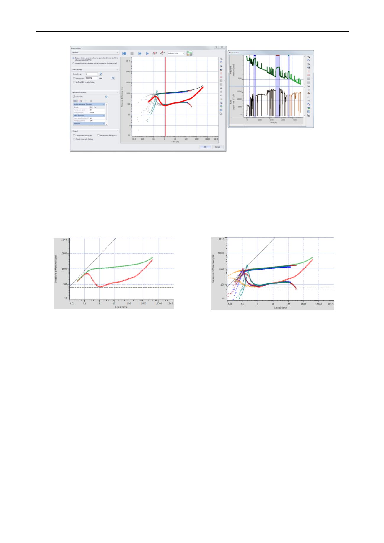
Fig. 3.D.25 – Deconvolution on one period as reference and reconvolved data
The Pi can be forced to a fixed value to improve the process efficiency.
The rate history correction can be desactivated.
It is possible to superimpose the deconvolved signal and the individual build-up data in a rate
normalized way. The reconvolved responses corresponding to the build-ups can also be
plotted.
Fig. 3.D.26 – Deconvolved response
Fig. 3.D.27 – Compared to BU data
and reconvolved response
3.D.6
Using sensitivity to assess the validity of a deconvolution
The early time part of the deconvolution response is constrained by the build-up data, and the
tail end is adjusted to honour other constraints, such as the pressure drop between the
successive build-ups. When no constraint is applicable to a part of the data, the deconvolution
picks the smoothest possible path to minimize the curvature. There may be intermediate
boundary effects in the ‘real’ reservoir, but we have no way to know. An issue is to assess
which part of the deconvolved data is positive information, and which part is just a smooth
transition between positive information.
This is a very serious issue, and may be one of the main dangers of the deconvolution process.
When we interpret data and choose the simplest model that honors whatever we have, we
know the assumptions we make. When we add a closed system to a model matching individual
build-ups in order to reproduce the depletion, we know that we are taking the simplest model,
but that there may be additional and intermediate boundaries that we may not see. In its
apparent magic, deconvolution presents a long term response that is NOT positive information
but just a best match. So how can we discriminate positive information and information by
default?