KAPPA DDA Book v5.12

88 / 743

Dynamic Data Analysis – v5.12.01 - © KAPPA 1988-2017 Chapter - p88/743
How does this work?
We had 400 hours of production and 100 hours of shut-in. Deconvolution is attempting to
provide 500 (theoretical) hours of constant production. The first 100 hours of the spline
representation are rigid, because they have to match the build-up. We have a loose tail
between 100 and 500 hours. The regression moves the tail up or down in order to match the
initial pressure pi after superposition, i.e. to match the depletion during the producing phase.
If the initial pressure is higher than the infinite case, the depletion is greater, and the reservoir
has to be bounded. If the initial pressure is lower, the depletion is less and the derivative of
the deconvolution will tail down and exhibit pressure support.
Now, there are hundreds of tail responses that could produce a specific depletion. Which one is
picked? The simplest one, because the regression selects the solution with the lowest
curvature, i.e. the one that will go smoothly from the part of the response that is fixed to
whatever PSS level. The first part of the data is rigid, the last part is more or less set by the
depletion and the transition is as smooth as possible.
Naturally, if we had more intermediate data, like some reliable flowing pressures, this would
‘firm up’ the deconvolution algorithm. The optimization first focuses on matching the data
before trying to get a smooth response.
3.D.5.a Implementation in Saphir 5
The implementation in Saphir gives access to two of the above mentioned methods, through a
very logical workflow.
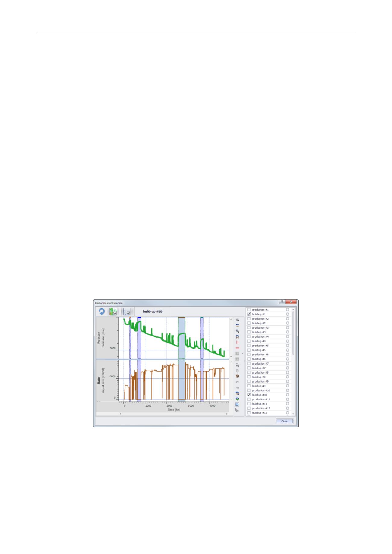
The periods to analyze must be first selected for extraction, they may be picked interactively:
Fig. 3.D.24 – Selecting the periods
Having selected one or more build-up, when the deconvolution process is called its dialog
offers possible methods:
- Deconvolution on one period as reference, and the end of the other periods (Houze et
al.)
- Separate solutions with a common Pi (Levitan et al.)