


 87 / 743

Dynamic Data Analysis – v5.12.01 - © KAPPA 1988-2017
Chapter
3 – P ressure Transient Analysis (PTA)- p87/743
3.D.5
Pi influence on the deconvolution
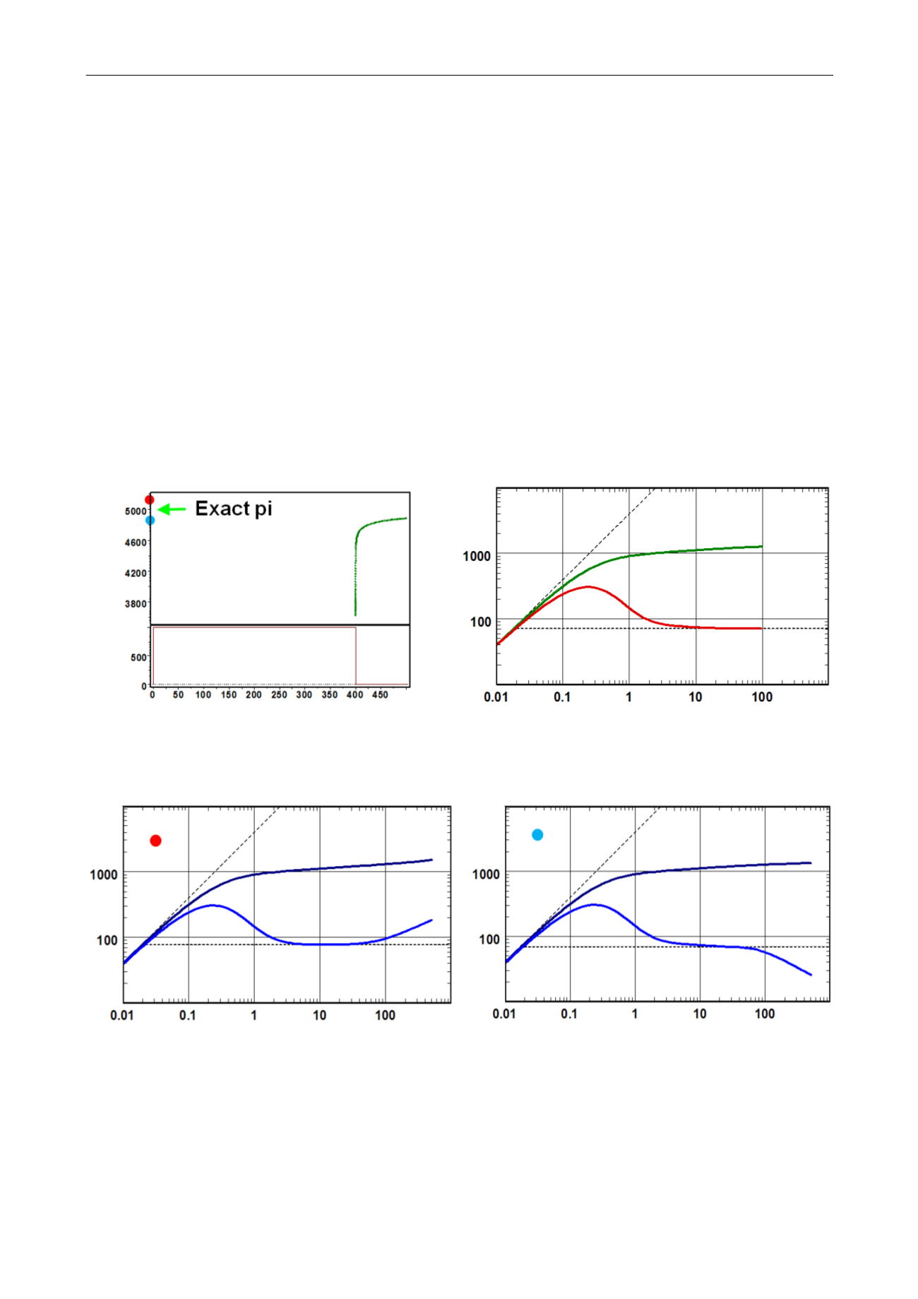
In the case illustrated in the figures below, we have run a test design with a homogeneous
infinite model. So we know that the right response is homogeneous infinite. It starts from an
initial pressure of 5,000 psia. There was a 400 hours constant rate production period followed
by a 100-hours shut-in.
When the deconvolution is run with too high a value of pi (red dot), there is an additional
depletion compared to the infinite case. In order for the deconvolution to honor both the build-
up and the initial pressure, it will have to exhibit at late time an increase of the derivative
level, typical of a sealing boundary. Conversely, if we entered too low a value of pi (blue dot),
there needs to be some kind of support to produce depletion smaller than the infinite case. The
deconvolution will exhibit a dip in the late time derivative.
In other words, deconvolution honors the data of the first 100 hours of the build-up, and then
uses the flexibility of the 400 last hours to ‘bend’ in order to be compatible with the entered
value of pi. Why is the shape so smooth? Because, on top of this, the optimization process
minimizes the total curvature of the derivative curve.
Fig. 3.D.22 – Deconvolution of a single build-up with different values of pi
For an infinite reservoir - Left: Simulation; Right: extracted build-up
Fig. 3.D.23 – Deconvolution with pi too high (red) or too low (blue)