


 32 / 743

Dynamic Data Analysis – v5.12.01 - © KAPPA 1988-2017
Chapte
r 2 – T heory- p32/743
2.F
Complex production histories – Superposition in time
2.F.1
The principle of superposition
Derivations as shown before assumed a constant rate production. In practice we need to
model more complex flow histories. This is done using the principle of superposition. We
generate the solution of a complex problem as the linear combination and superposition, in
time and/or space, of simpler components. The most popular superpositions are:
Simulation of complex production histories by linear combinations of simple drawdown
solutions with different weights and starting times. This is called superposition in time, the
equations are developed in the chapter ‘Analytical models - 13.C - Superposition in time’.
Simulation of simple linear boundaries by linear combinations of infinite well and
interference solutions coming from virtual wells (also called image wells).
For any problem involving a linear diffusion equation, the main superposition principles are:
Linear combinations of solutions honoring the diffusion equation also honor this equation.
At any flux point (well, boundary), the flux resulting from the linear combination of
solutions will be the same linear combination of the corresponding fluxes.
If a linear combination of solutions honors the diffusion equation and the different flux and
boundary conditions at any time, then it is THE solution of the problem.
A series of rules for superposition in time are built from these principles, they are detailed in
the chapter ‘Analytical models - 13.C - Superposition in time’.
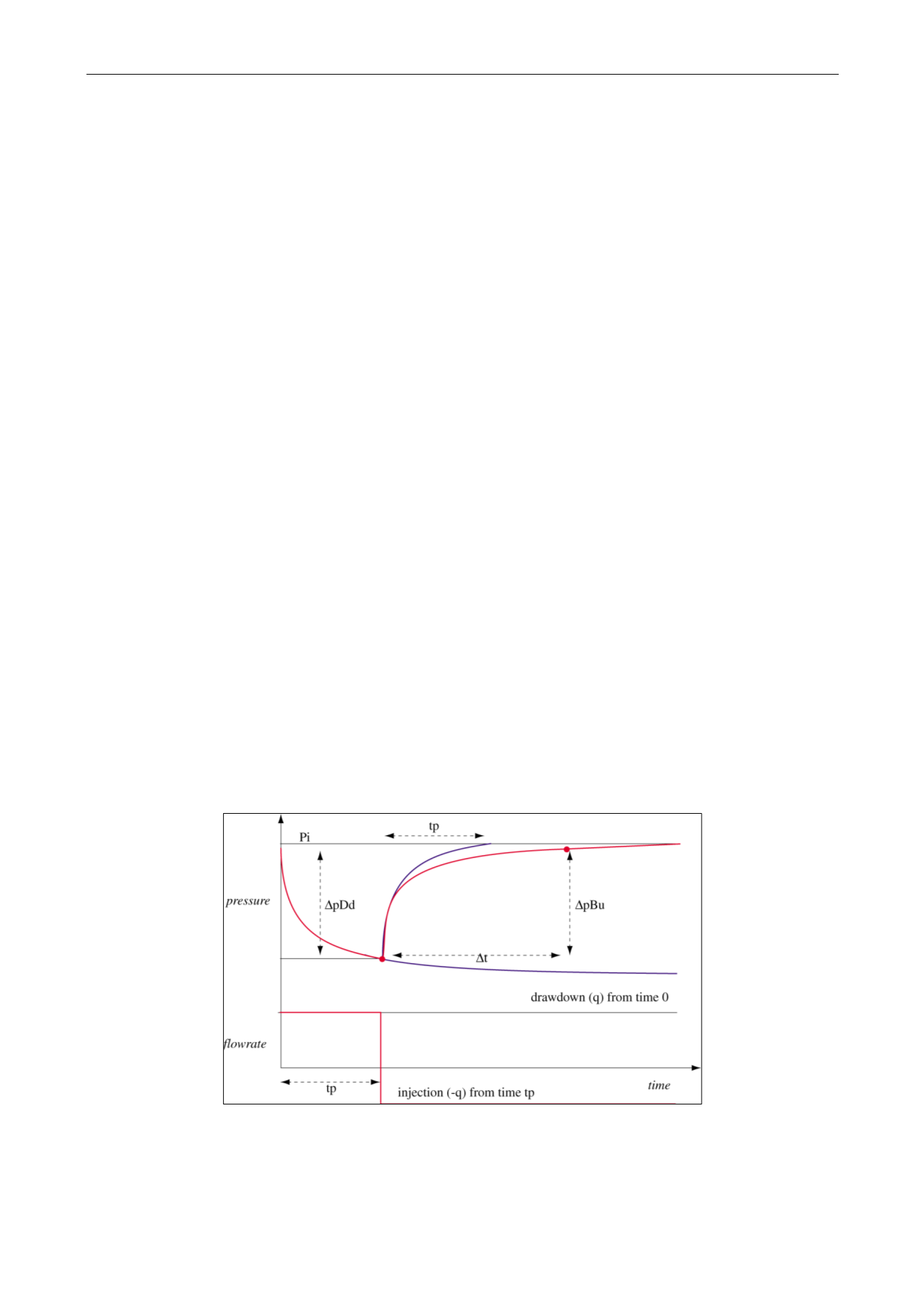
2.F.2
Build-up superposition
We consider a production at rate q of duration t
p
, followed by a shut-in:
Fig. 2.F.1 – Buildup superposition