


 31 / 743

Dynamic Data Analysis – v5.12.01 - © KAPPA 1988-2017
Chapte
r 2 – T heory- p31/743
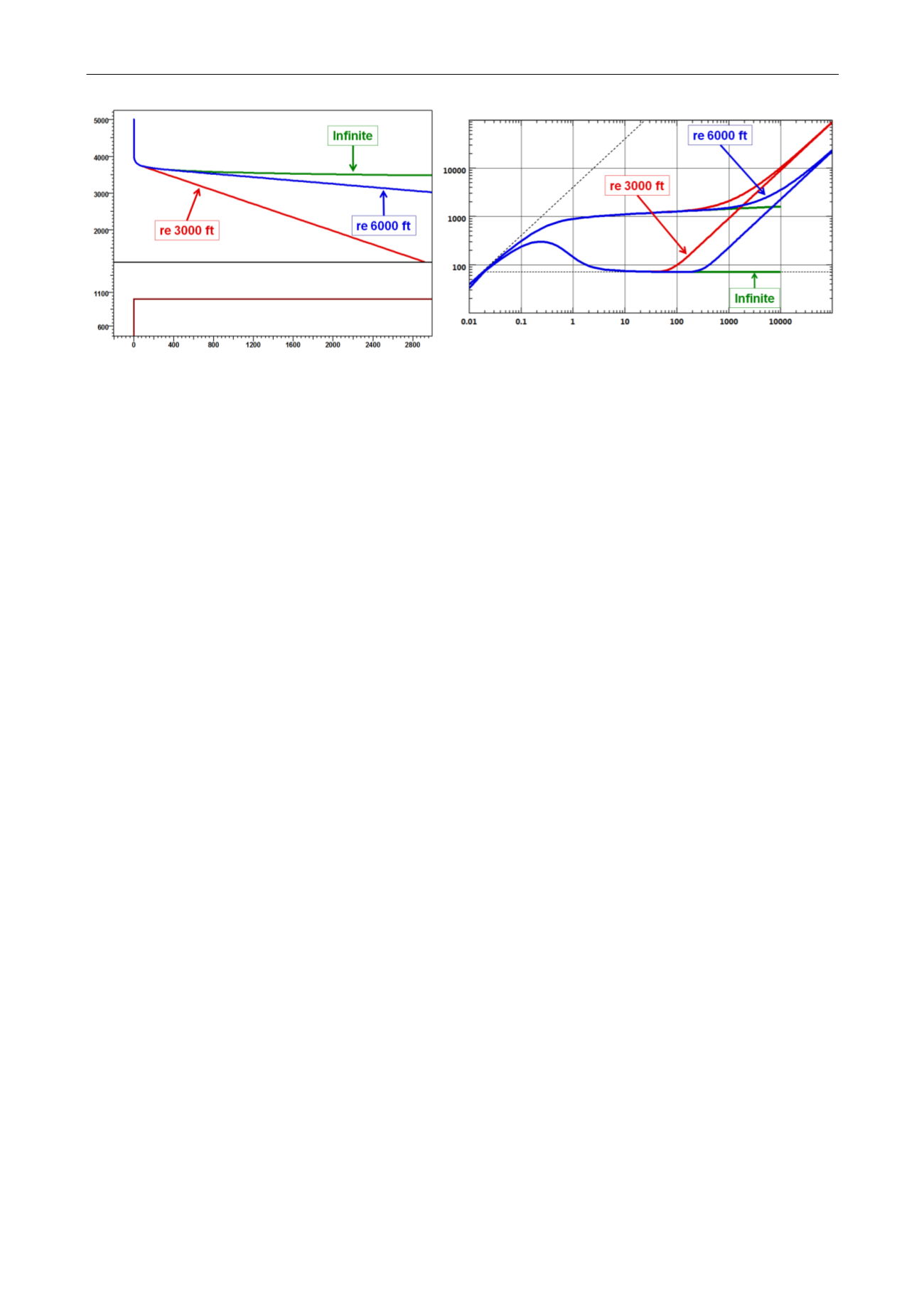
Fig. 2.E.2 – Finite radius PSS solution,
Fig. 2.E.3 – Finite radius PSS solution,
linear scale
loglog scale
Comparing the two circular responses:
Drawing a straight line on the linear plot will show that the slope of the ‘re 3,000 ft’ line is
twice larger than the slope of the ‘re 6,000 ft’ line.
Looking at the time of deviation from IARF on the loglog plot, we see that this occurs 4
times earlier for the 3,000 ft case than for the 6,000 ft case.
In both cases we see the inverse proportionality of the slope and the time of divergence to the
square of the reservoir radius or, more generally to the reservoir area.
The circular model is only one example of closed systems, and Pseudo-Steady State exists for
all closed systems. It is a regime encountered after a certain time of constant rate production.
Although it is a flow regime of interest for Pressure Transient Analysis, it is THE flow regime of
interest in Rate Transient Analysis. Pseudo-Steady State may sometimes not only be seen as a
result of reaching the outer boundary of the reservoir; in a producing field, for example, there
is a time when equilibrium between the production of all the wells may be reached, and, for
each well, Pseudo-Steady State will occur within the well drainage area.
For a slightly compressible fluid, Pseudo-Steady State is characterized by a linear relation
between the pressure change and the time. When PSS is reached, the pressure profile in the
reservoir will ‘freeze’ and the pressure will deplete linearly and uniformly throughout the
connected reservoir. Things are somewhat different when the PVT becomes complex.