Carbone is a highly interactive package designed to build, tune and operate on EoS or Black Oil fluid models. Whilst the simplest use case may be to build a PVT model for KAPPA-Workstation or any other Black Oil or
Compositional modeling platform, Carbone is designed to be used for more advanced applications in reservoir, production and flow assurance domains.
These include constructing a field or asset scale unified EoS model, Wax, Asphaltene, Hydrate and Salt precipitation studies, compositional gradient calculations, miscibility pressure calculations, surface unit modeling and design, shrinkage calculations, separator optimizaiton and production allocation.
With speed and ease of use at its core, processes such as fluid and lab data QC, phase envelope generation, flash results and model comparison are automatically performed for any fluid.
Carbone is powered by the technical kernel from IFPEN as part of our ongoing technical partnership.
Built as part of KAPPA Generation 6, Carbone has a web UI and separate back end, allowing various deployment configurations, namely stand-alone, client-server, or through the KAPPA-Automate platform as a microservice.
Carbone offers a multilingual UI, currently supporting English, French, Russian, Chinese and Spanish.


Fluid Definition
Carbone offers an extensive, customizable and extendable internal database of pure and pseudo components to define a fluid.
Twu/Edmister, Lee-Kesler Extended, Riazi/Edmister and Pedersen correlations are available to compute pseudo component properties from Mw, S.G and/or Tb.
In addition to selecting components and defining the composition and properties of a fluid in Carbone, fluids may also be initialized by importing files in Eclipse™ compositional format.
EoS models
Carbone offers the following EoS models:
1. Peng-Robinson, 1978
2. Soave-Redlich-Kwong, 1972
Pseudo component acentric factors and volume shifts may be constrained to component boiling points and component surface densities respectively.
Note: There are additional EoS models implemented in Carbone, but their usage is restricted to specific fluid types only. These include:
3. GERG-2008: Available to a dedicated component library.
4. Abdoul-Rauzy-Peneloux (ARP), 1991: Asphaltenes only
5. Cubic Plus Association (CPA): Fluid phase in Hydrates
6. Søreide-Whitson, 1992: 3-phase aqueous flash calculations
Viscosity model
The following viscosity models are available:
1. Lohrenz-Bray-Clark, 1964 (LBC)
2. LBC Heavy Oil
3. Little & Kennedy, 1968
4. Pedersen, 1987 (Corresponding State Principle, CSP)
5. Pedersen, 2014
6. Ducoulombier, 1986 (adjustement to Pedersen's CSP model for heavy oils)
Critical volumes may be constrained to the Orrick & Erbar, 1973 correlation when using the LBC correlation.
Phase Envelope & Flash Results
A PT phase envelope is simulated on the fly for any fluid. Multiple phase envelopes can be compared.
Flash results, including mixture properties, oil and gas phase composition, thermodynamic, transport and thermal properties are automatically computed and output at reservoir and standard conditions.
Users can also specify additional pressures and temperatures at which to compute flash results.
3-phase Aqueous Flash
The Søreide & Whitson, 1992 model is used for 3-phase aqueous flash. This model is based on the Peng-Robinsion EoS, with the following modifications to improve predictions in the presence of water:
1. Using a modified α-term in the EOS constant a for the brine component as a function of water reduced temperature and brine salinity.
2. Using two sets of BIPs for each binary including water/ brine kijAQ and kijNA for the aqueous phase and non-aqueous phase, respectively.
kijAQ is expressed as a function of NaCl brine salinity, hydrocarbon acentric factor and reduced temperature. For kijNA a constant value is applied, except for H2S.
Water-Oil Emulsions
If a 3-phase Aqueous Flash has been performed, the following models are available to estimate emulsion viscoity:
1. Woelflin
2. Smith & Arnold
3. Guth & Simha
4. Brinkman
5. Volumetric
6. Continuous phase
The critical water cut may be estimated using either of the following models:
1. Arirachakaran
2. Brauner & Ullmann
3. Brinkman
4. Constant
Sample/Lab Data QC
The following QC methods are available for sample composition and the different lab experiments:
1. Auto-screening of sample composition for OBM contamination
2. Oil density mass balance
3. Composition forward material balance / Bashbush plot
4. Composition backward material balance
5. Z-Factor comparison with Standing & Katz chart
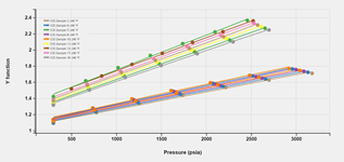
6. Y-Function plot for CCE, DLE and CVD experiments
7. Hoffman plot
8. Inequality Test
9. Comparison of CCE and CVD LDO curves
Additionally, users can compare different experiments for a given fluid or across multiple fluids within a Carbone document. When comparing experiments, relevant QCs are also compared.
Handling Lab Data Uncertainty
A default table of user editable relative uncertainty in common experimental data is built into the application. These values are displayed as error bars on the different plots, aiding users with assessing data consistency and quality of match between the EoS simulation and data.
These uncertainties are also accounted for when color coding the quality of match between simulated and experimental data.
Characterization/EoS Model QC
Carbone offers a wide range of options to QC a given fluid/characterization at any stage in the workflow. They fall in two categories: Category 1 QCs raise warnings;
Category 2 QCs rely on different plots which are readily available to the user to view. However, no warning is issued, and the user must manually consult these plots to verify model consistency. All QCs are automatically and always
performed on all fluids in a document.
These methods are listed below ((W) for Category 1 QCs, which raise warnings):
1. Fluid phase at Reference Temperature.
2. Phase change during regression (W).
3. Potential OBM contamination (W).
4. Psat > Pref (W).
5. Non-monotonic pseudo-component Pc, Tc or Vc (W).
6. Pseudo-component Tb outside Katz-Firoozabadi SCN range (W).
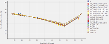
7. Component property vs. Mw plots.
8. Equilibrium Ratio vs. Pressure and vs. Tb plots.
9. Comparison with lab data: No particular warning is issued, but the errors automatically (and always) calculated and color-coded:
Green if difference < 5%, Orange if difference between 5 - 10% and Red if difference > 10%.
Decontamination
For samples which may have been contaminated by Oil Based Mud (OBM), two methods are available to ‘clean’ the sample composition:
1. Skimming: Assumes an exponential molar distribution model for the uncontaminated fluid; used when the mud composition and contamination are not known.
2. Subtraction: used when the mud composition and contamination are known.
An automatic screening is performed on the sample composition to check for possible contamination. If suspected, a warning is issued to the user:
Characterization
A detailed, multi-sample, field-wide characterization can be carried out in Carbone. The process steps include:
1. Molar Distribution Models: Choose between Exponential or Gamma distribution models and tune model parameters to match a single or multiple samples
2. Characterization Factors: Correlate molecular weight and specific gravity of one or multiple samples from a field using Watson, Jacoby or Søreide Characterization Factors.
3. Boiling Point Estimation: Correlate pseudo-component molecular weight and boiling points using Twu or Søreide correlation.
The tuned characterization can help QC any bad quality GC data and systematically replace bad quality GC data with reliable estimates from the model. In the absence of extended GC data, the plus fraction can also be split
into heavier fractions from the characterization.
Once a characterzation is created, it can be applied to any compatible fluid, allowing users to develop field-wide EOS models.
Split
Carbone offers two Split options for the plus fraction:
1. Standard split: Split the plus fraction to C80 (Conventional oil & gas condensate) or C200 (Heavy oil) assuming an exponential distribution (Pedersen et al., 1983 and 1984)
and lump back to a user-defined number of components, based on equal mass lumping method of Pedersen, 1984.
2. Split to Cn+: Similar to (1), except that the split is done to a user-defined Carbon Number (CN). No lumping is done after the split.
Lumping
Lumping is used to reduce the number of components of a given fluid. The following lumping methods are available:
1. User defined: groups of components are created by the user. Carbone computes the equivalent properties of these components and assigns them to the groups.
2. Montel Gouel: a target number of components is specified by the user. Carbone automatically groups and computes the components using the method proposed by Montel and Gouel, 1984.
3. SARA: This is an automatic lumping scheme, derived from the method proposed by Scewczyk et al., 1999, to recharacterize an existing fluid for Asphaltene modeling using SARA information.
Optimized Lumping
The objective of Optimized Lumping is to find the most appropriate lumping scheme to describe a set of processes, given a target number of required components. An example could be the following: Lump a 40-component fluid to a 6-component fluid, which matches the saturation pressure and flash results of the 40-component fluid as close as possible.
Two optimization algorithms are available in Carbone:
1. Brute Force: Derived from Alavian et al. (2014). All combinations of lumping are evaluated.
2. Genetic Algorithm: Derived from Hoffman (2019). A genetic search is performed followed by a Tabu search..
Regression Types & Variables
Nine kinds of regression types are available:
1. Classical pseudo regresses on the following pseudo component properties: Tc, Pc, ω/Tb, Volume Correction/Specific gravity and Kijs.
2. Primary Variables on pseudo component Tb and Specific Gravity, with automatic recomputation of all derived properties.
3. EoS parameters on Ωa and Ωb parameters.
4. Viscosity Model on Critical Volumes and Modified LBC parameters.
5. Automatic Heavy, on the boiling point of the heaviest fraction to match on the liquid density at standard conditions.
6. Mw+, on molecular weight of pseudo-components.
7. Recombination, on flash gas-oil recombination ratio.
8. Asphaltene, on Tc and Molecular weight of Asphlatene fractions.
9. Wax, on Melting Point, Enthalpy of Fusion of Wax fractions and Pedersen Viscosity model coefficients.
Two gradient based solvers are available for regression: KAPPA and Hubopt.
Regression Targets
Any lab data associated to a given fluid may be used as regression targets. The granularity of target selection is down to individual measurements points.
Relative weights can be assigned to entire experiments or part of an experiment to customize the objective function.
If compositions have been loaded for different depletion experiments, they can be also included in the objective function for regression
Multi-sample Lab Data Management
Flexible lab data management allows users to compare different experiments for a single sample or across multiple samples loaded in a given Carbone document. Among other things, this facilitates users to:
1. Identify data trends
2. Identify outliers
3. Identify potential groupings
which allows users to gain better insights in to the different data available and aid in the QC of lab data at a field or asset level.
When comparing experiments, any relevant QCs are also compared:
Multi-sample Fluid Management
Flexible fluid management allows users to compare and visualize information contained across multiple samples in a given Carbone document. These include:
1. Sample compositions
2. Component properties
3. Component equilibrium ratios
4. Phase envelopes
5. Flash results at reference or user defined conditions
which allows users to gain better insights in to the different samples at a field or asset level.
Unified Multi-fluid Characterization
Part of the unified EoS development workflow is to use all (or a subset of) available compositions and surface oil density data to arrive at a single characterization for all samples in a given field or asset.
The characterization workflow (detailed under 'Characterization' above) can be easily scaled to multiple samples to achieve this using only a few clicks.
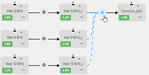
Unified Multi-Fluid Regression
Once a common characterization is built for multiple fluids, a global regression can be run on them. Each fluid will use its composition to match its lab data, while maintaining a unique characterization across all the fluids.
The regression options (detailed under 'Regression' above) can be easily scaled to multiple samples to achieve this using only a few clicks.
Constrained Split and Lumping
Once a common characterization is built for multiple fluids, the same split or lumping can be applied to all of them by enabling the 'Constrained split' or 'Constrained lumping' option in the respective dialogs.
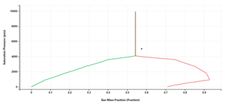
Miscibility Pressure
Minimum and First Contact Miscibility Pressure (MMP/FCMP) may be calculated between an original and an injection fluid. The injection fluid may be single or multi-component.
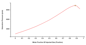
The calculations in Carbone are based on Neau et. al., 1996. The main benefit of this approach is that MMP is directly computed, without successively simulating Vaporizing and Condensing Drive Mechanisms.
Compositional Gradient
The compositional gradient process calculates the variations in composition and properties of a reservoir fluid as a function of reservoir depth. The method in Carbone is based on Montel & Gouel, 1985.
Properties and Compositions from multiple gradients can be compared with each other as well as with any loaded versus depth log.
For any depth, compositions can be output as a new ‘Fluid’ on which any process may be applied.
Surface Units Modeling and Design
The following surface units can be modeled:
1. Separator
2. Heater
3. Pump
4. Compressor
5. Valve
It is also possible run multiple sensitivities on input parameters and study their impact on surface unit outputs.
Fluid Mixing
Two fluid streams may be mixed together based on:
1. Target GOR
2. Mole Fractions
3. Volume Fractions at a given P, T
Well Test Match
Producing wellstream compositions can change over time. The Well Test Match option can calculate an updated composition (from the seed composition) to match measured GOR, Oil Density and Gas Gravity.
Shrinkage Calculation
In the absence of direct stock-tank measurements, the shrinkage option can be used to reliably convert oil rates, measured at test/line conditions to standard conditions.
There are two main inputs to these calculations:
1. Device information: Pressure, Temperature and measured Oil and Gas rates
2. Separator information: Pressure and Temperature of different separator stages in the production/processing facility
The results of these calculations are:
1. Well stream composition, honoring device production ratios
2. Fluid composition at each separation stage
3. Oil and gas rates and properties at each separation stage
4. Shrinkage value
Separator Parameters Optimization
An extension to the shrinkage calculation option, this option allows separator pressure and temperature optimization to minimize shrinkage (maximize liquid yield) over a given number of separator steps.
Production Allocation
The objective of these computations is to allocate to individual well streams feeding into a processing facility the fraction of the stock tank volumes (qkGAS, qkOIL) produced from the processing facility (qGAS, qOIL).
The inputs needed for this computation are:
1. Metering conditions - Pressure and Temperature.
2. Production rates of each stream at metering conditions (gas rate may be input at metering or standard conditions) - qkgas, qkoil.
3. Processing facility set up - Pressure and Temperature of each separator.
The method proposed by Pedersen (2005) is used to perform the allocation.
The outputs this computation are:
1. A schematic illustrating the process i.e., mixing of the different fluid streams and the 'Feed' stream processing through the production system.
2. Results Table showing the oil and gas rates allocated to the individual well streams.
3. Fluid Results table showing the fluid volumes and properties at each node in the schematic.
4. Fluid Composition showing the composition of the fluid(s) at each node in the schematic.
Wax
Carbone provides an automatic PNA split scheme for Wax Characterization based on the method proposed by Nes & Westerns, 1951. The characterization can be based on Cmin, Cmax range of wax forming SCNs or Cmin and total wax amount (from which Cmax is iteratively computed). Users can specify which of the three component families will be part of the solid phase.
The Wax Model in Carbone is derived from the one proposed by Pedersen, 1995. The solid phase is assumed to behave ideally.
WAT and Wax Precipitation curves are automatically generated for any ‘Wax’ fluid.
The Wax Viscosity model is derived from Pedersen and Rønningsen (2000), which allows computation of Fraction of Crystallized Wax (ɸwax) vs. shear rate from Apparent Liquid Viscosity (ηapparent) vs. shear rate data. Plots of both ηapparent and ɸwax are displayed vs. shear rate.
A dedicated Wax Regression offers tuning on Melting Point and Enthalpy of Fusion of the Wax forming components to match WAT, Wax precipitation and/or Wax Viscosity data.
Note: other regression types can also be used for a Wax fluid.
Asphaltenes
Asphaltene Characterization is based on an automatic lumping process, which lumps any fluid into a 10-component ‘Asphaltene’ fluid, based on SARA input. The method is derived from Scewczyk et al., 1999.
The following methods are available for Asphaltene Risk Assessment:
1. De Boer's method (De Boer et al., 1995)
2. Colloidal Instability Index (CII) method (Yen et al., 2001)
3. Stankiewicz Asphaltene Stability Index (ASI) method (Stankiewicz et al., 2002)
The Asphaltene Model treats Asphaltene as a solubility class and models asphaltene precipitation as Liquid-Liquid demixing. Abdoul et al., 1991 equation of state is used to analyze the various phases.
The entire Asphaltene phase envelope for the complete PT spectrum is automatically generated. Additionally, Asphaltene solubility, Asphaltene precipitation, oil density and solid density curves are automatically generated for any ‘Asphaltene’ fluid.
A dedicated Asphaltene Regression offers tuning on Tc and Mw of the Asphaltene components to match the asphaltene onset pressure and/or precipitation data.
Note: other regression types can also be used for an Asphaltene fluid.
Hydrates
Hydrate structures of type S1 and S2 can be defined. Impact of Methanol, Ethanol and MEG on hydrate phase envelope can be modeled.
For a given setup and additive amount, crystallization temperature at a given pressure (and vice versa) can be calculated.
In addition, Hydrate composition and stability graph with and without the additive is also output. Different inhibitor types and concentrations can thus be studied.
The Hydrate Model uses the approach proposed by van der Waals and Platteeuw, 1959 and extended by Parrish and Prausnitz, 1972 for the Hydrate phase and the Cubic Plus Association (CPA) Equation of State for the fluid phase.
Scales/Salts
The following common salts can be modeled in Carbone: NaCl, CaSO4, BaSO4, SrSO4, CaCO3, FeCO3 and FeS.
Two approaches are available for modeling of scale precipitation:
1. Scaling Tendencies (Qualitative Model).
2. Mineral Precipitation (Quantitative Model).
The Qualitative model provides a Saturation Index (SI) of the different salts which may form in solution at different Pressures and Temperatures. The SIs are plotted versus Pressure and Temperature for the different salts.
The Quantitative model calculates the amount of mineral precipitation at different Pressures and Temperatures. The amounts of precipitated salts are plotted versus Pressure and Temperature for the different solids.
The calculations are made via a Non-Stoichometric Reactive Flash algorithm. The vapor phase is modeled by a Cubic EoS. The aqueous phase is modeled by the Pitzer Activity Model and each solid phase is assumed to be pure and ideal.
Experiment Design
The Experiment Design tool allows users to generate experimental data for any compositional fluid.
Fluid Definition
Fluids properties can be defined using a broad range of Black Oil correlations (see Technical References). These correlations can also be tuned to user data.
Alternatively, properties may be defined from user tables.
A Black Oil fluid may also be initialized from either KAPPA or Eclipse™ BO files.
Fluid Types
The following Black Oil fluid types can be created:
1. Dry Gas (Hydrocarbon, Pure N2 or Pure CO2)
2. Wet Gas
3. Condensate
4. Dead Oil
5. Saturated Oil
6. Volatile Oil
Water can be included with any of the fluid type.
Flash Results
Flash results, including mixture properties, oil and gas phase thermodynamic and transport properties are automatically computed and output at reservoir conditions.
Users can also specify additional pressures and temperatures at which to compute flash results.
A P-x phase envelope is simulated on the fly for Modified Black Oil formulation (Condensate and Volatile Oil Fluid Types).
Multiple phase envelopes can be compared.
Export Compositional Fluid
Carbone offers the following compositional formats to export fluid PVT:
1. XML compositional (for KAPPA applications)
2. Eclipse™ compositional
3. Intersect™ compositional
4. PROSPER™ compositional
5. CMG compositional (STARS™ and GEM™)
6. OLGA: EoS CTM, EoS TAB and Wax Table
Generate Black Oil Tables
Black oil tables can be generated for a compositional fluid and exported in one of the following formats:
1. KAPPA BO
2. Eclipse™ BO and GI
3. Intersect™ BO
4. CMG BO (IMEX™)
BO properties are generated using the method of Whitson and Torp, 1983. Reservoir depletion processes can be modeled using CCE, CVD or DLE. Surface separator systems can be defined for the export.
Black Oil Fluid
Properties for black oil fluids may be exported in tabular format.
Additionally, an XML output of the black oil fluid setup can be created for easy transfer to other KAPPA modules.
Workflow Integration
Compositional or Black Oil PVT can be exchanged with any KAPPA-Workstation module through a simple Drag and Drop via the KAPPA-Workstation browser.
Additionally, a Carbone document stores all the objects and results of a given session in a human readable JSON structure. This facilitates users to write their own scripts to access any data in a given Carbone document
and integrate it within their workflows.