Page 9 - Numerical Multiphase PTA

VA – GP - OA: Numerical Multiphase PTA p 7/29
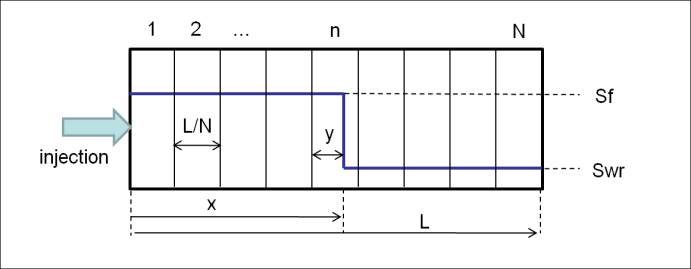
Let us now discretize this model by introducing N cells in the problem (Figure 8).
Figure 8: 1D displacement with the discrete model
In the discretized model, the position of the front within a cell is not accessible, and only the
average saturation in the front cell w S is used. The pressure drop becomes:
 
   
 
  






 
 


wr t w t f t S
nN
S S
n
CP
  
1 1
. (Eq A)
w S can be expressed in function of the position of the front as:
     
NL
xy NL S xy S
S wr f
w /
/    
 (Eq B)
Obviously, w S is still a linear function of x. However, the total mobility  w t S  can be very non-
linear, as shown previously on Figure 4. This explains the development of oscillations.
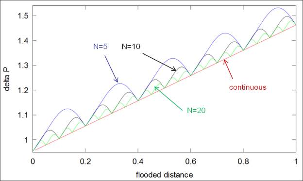
On Figure 9, the expression for the pressure drop in the discretized model has been solved as
a function of the position of the front (Eq A and Eq B with arbitrary values L=1 and C=1), for
various discretization levels N. Each oscillation corresponds to the invasion of a new cell during
the displacement.
Figure 9: Oscillations obtained with the discrete model, for various discretization levels
From this model, we see that increasing the number of cells reduces the amplitude of the
oscillations and increases their frequency, as was observed with Test Case 1.