Basic HTML Version


Ecrin v4.12 - Doc v4.12.02 - © KAPPA 1988-2009
Topaze Guided Session #2
•
TopGS02 - 9/12
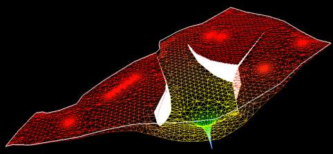
The animation can also be seen in pseudo 3D. Click on
. You may have to use the zoom
options
in order to get a similar screen as the one shown in Figure B02.7.
To show the surface, click on the 3D Plot Settings icon
to
enable the 'show surfaces' option
of the Settings tab.
The following figure illustrates the same time field as Figure B02.6.
Fig. B02.7 • 3D geometry plot
Click on to switch back to 2D.
Double click on the Analysis tab name 'Analysis 1' and change the name to 'Single Well'.
Duplicate the current analysis by clicking on the
tab. Accept the default to start from
the current analysis and name it ‘2 Wells’.
Return to the 2D Map tab. We will enter a production history for a second well only, the
producer named P05.
Double click on this Well, select its Pressures tab, then Load. Choose 'Keyboard – spreadsheet'
and enter the following pressure history (expressed in hours and psia):
500-3000;
500-2000
, click on ’Next‘ and specify 'Steps: durations'. Click on ’Load‘. Accept the default
value in the ‘Set Initial Pressure’ dialog.
Go to the ‘2 Wells’ analysis tab and click on Model. The 'add other wells' button is now
available. Select this option and Generate, Figure B02.8.